Elliptic3D.edp

Resumen: En este ejemplo se considera un problema eliptico en dimensión 3.

Problema

Consideramos el problema:

\begin{matrix} (1) & {\begin{cases} - \nabla \cdot (A \nabla u) + c u = f & en Ω, \\ u = g & sobre Γ_{1} \cup Γ_{2}, \\ (A \nabla u) \cdot n = h & sobre Γ_{3} . \end{cases} \end{matrix}

$\Omega$ $\mathbb{R}^3$ $\Omega = (0,1)\times(0,2)\times(0,0.5)$ $c\in\mathbb{R}$ $A =(a_{ij})_{i,j=1}^{3}$ es una matriz de coeficientes reales simétrica.

$\Gamma_1$ $\Gamma_2$ $\Gamma_3$ son los lados).

Formulación débil

$V = \{ \mathbf v\in H^1(\Omega) \,\colon\, \mathbf v = 0 \quad\text{sobre}\quad \Gamma_1\cup\Gamma_2\}$ .

$\eqref{eq.elliptic3D.1}$ $\mathbf v\in V$ $\Omega$ , y utilizando la integración por partes, se llega a la siguiente formulación débil o variacional del problema:

\begin{matrix} (2) & {\begin{cases} Hallar u \in \tilde{g} + V tal que \\ \int_{Ω} (A \nabla u) \nabla v d x d y d z + \int_{Ω} c u v d x d y d z - \int_{Ω} f v d x d y d z - \int_{Γ_{3}} h v d σ = 0 \forall v \in V . \end{cases} \end{matrix}

$c = 5$ $f=\mu_0 \, e^{-|\mathbf{x}-\mathbf{p}|^2/2\sigma_0}$ $\mathbf{p} = (0.85, 1.7, 0.25)$ $\mu = 1$ $\sigma_0 = 0.025$ y

\begin{matrix} \begin{matrix} A = (\begin{matrix} 10 & 0 & 0 \\ 0 & 10 & 0 \\ 0 & 0 & 10 \end{matrix}) . \end{matrix} \end{matrix}

$f$ $\mathbf{p}$ $\nabla f$ sea "grande". Por ello, realizamos una adaptación del mallado 2D antes de construir, por capas, el mallado del dominio 3D.

Código


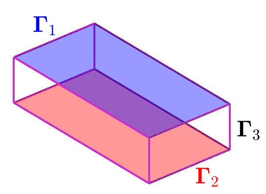
//  3D elliptic equation with Dirichlet and/or Neumann cond.
//  | - \nabla\cdot(A\nabla u) + c u = f,  x \in \Omega
//  |     u = g,   x \in \Gamma_1 \cup \Gamma_2 (top and bottom)
//  |    (A\nabla u) \cdot n = h,   x \in\Gamma_3 (sides)
//
//      \Omega = (x_0,x_1) \times (y_0,y_1) \times (z_0,z_1)

//  Description of the variables
//  x0, x1, y0, y1, z0, z1                : limits of the domain
//  a11, a12, a13, a22, a23, a33, c0      : coefficients of the pde
//
load "msh3"        // for 3D meshes 
verbosity = 0;

//
//  Data
//
real x0 = 0., x1 = 1.;                    // $x_0$, $x_1$
real y0 = 0., y1 = 2.;                    // $y_0$, $y_1$
real z0 = 0., z1 = 0.5;                   // $z_0$, $z_1$
real a11 = 10., a22 = 10., a33 = 10.;     // pde coefficients
real a12 = 0., a13 = 0., a23=0., c = 5.;  // pde coefficients
real mu0 = 1., sigma0 = 0.05;            // coef. of gaussian function
real sigma = -0.5/sigma0;
real px=.15*x0+.85*x1, py=.15*y0+.85*y1, pz=.5*z0+.5*z1;  // point in the domain

func f = mu0*exp(sigma*((x-px)^2+(y-py)^2+(z-pz)^2));  // RHS
func g = 0.;                                           // Dirichlet data
func h = 0.;                                           // Neumann data

//
//  Auxiliary data
//
real hx = x1-x0;
real hy = y1-y0;
real hz = z1-z0;
func f2d0 = mu0*exp(sigma*((x-px)^2+(y-py)^2));       // for mesh adapt.

//
//  Mesh
//
int nx = 5, ny = 5;                      // initial discret. along X, Y
int nz = 9;                              // number of layers
int L1 = 1, L2 = 8, L3 = 16;             // Labels
int[int] Lab =[L3,L3,L3,L3];
mesh Th2d = square(nx, ny, [x0+hx*x, y0+hy*y], flags = 3, label = Lab);
plot(Th2d, cmm = "First 2D mesh. Nb. vertex = "+Th2d.nv, wait = true);

//
//  Adaptive mesh
//  Adapting according to f2d0 function
Th2d = adaptmesh(Th2d, f2d0, hmax = 0.25, err = 0.005);
plot(Th2d, cmm = "Adapted mesh. Nb. vertex = "+Th2d.nv, wait = true);

//
//  3D mesh
//
int[int] rup   = [0,L1];
int[int] rdown = [0,L2];
mesh3 Th3d = buildlayers(Th2d, nz, zbound = [z0,z1],
                         labelup = rup, labeldown = rdown);
plot(Th3d, cmm = "3D mesh. Nb. vertex = "+Th3d.nv, wait = true);

//
//  Finite element space
//
fespace  Vh(Th3d, P2);
Vh u,v;
Vh fh = f, gh = g, hh = h;
plot(Th3d, fh, cmm = "Right Hand Side of the equation", wait = true);
//
//  Problem
//
problem Elliptic3D(u,v) = 
        int3d(Th3d)(
        a11*dx(u)*dx(v) + a22*dy(u)*dy(v) + a33*dz(u)*dz(v)
      + a12*(dx(u)*dy(v)+dy(u)*dx(v)) 
      + a13*(dx(u)*dz(v)+dz(u)*dx(v))
      + a23*(dy(u)*dz(v)+dz(u)*dy(v)) 
      + c*u*v)                             // bilinear
      - int3d(Th3d)(fh*v)
      - int2d(Th3d, L3)(hh*v)              // linear
      + on(L1, L2, u = gh)                 // boundary data
        ;
//  Solving the problem   
Elliptic3D;

//
//  Plots
//
plot(Th3d, u, cmm = "Solution", value=true, fill=true, nbiso=40, wait=true );

Anna Doubova - Rosa Echevarría - Dpto. EDAN - Universidad de Sevilla