Ecuación de ondas acoplada con ec. parabólica

Resumen: En este ejemplo se considera un problema relativo a la ecuación de ondas, en la aparece una función que, a su vez, es solución de una ecuación parabólica.

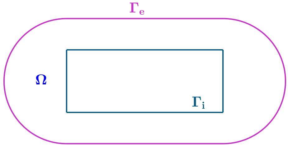
Problema considerado

$\Omega = \Omega \subset \mathbb{R}^2$ $T>0$ $u, \omega:\Omega\times(0,T) \to \mathbb{R}$ tales que

\begin{matrix} (1) & {\begin{cases} \partial_{t} u - a Δ u = f & en Ω \times (0, T), \\ \partial_{t t} w - c^{2} Δ w = b u & en Ω \times (0, T), \\ u = g_{e} & sobre Γ_{e} \times (0, T), \\ u = g_{i} & sobre Γ_{i} \times (0, T), \\ \frac{\partial ω}{\partial n} = 0 & sobre Γ_{e} \times (0, T), \\ ω = 0 & sobre Γ_{i} \times (0, T), \\ u (x, y, 0) = u_{0} (x, y) & en Ω, \\ ω (x, y, 0) = ω_{0} (x, y) & en Ω, \\ \partial_{t} w (x, y, 0) = w_{1} (x, y) & en Ω, \end{cases} \end{matrix}

$a,b,c\in\mathbb{R}$ $a>0$ $f:\Omega\times(0,T) \to \mathbb{R}$ $g_e:\Gamma_e\times(0,T)\to\mathbb{R}$ $g_i:\Gamma_i\times(0,T)\to\mathbb{R}$ $u_0, \omega_0, \omega_1: \Omega\to \mathbb{R}$ $\Omega$ es:

$\eqref{eq.tempwave2D.1}$ $u$ $\omega$ $u$ , resolviendo el problema:

\begin{matrix} (2) & {\begin{cases} \partial_{t} u - a Δ u = f & en Ω \times (0, T), \\ u = g_{e} & sobre Γ_{e} \times (0, T), \\ u = g_{i} & sobre Γ_{i} \times (0, T), \\ u (x, y, 0) = u_{0} (x, y) & en Ω, \end{cases} \end{matrix}

$\omega$ $u$ calculada en el segundo miembro de:

\begin{matrix} (3) & {\begin{cases} \partial_{t t} w - c^{2} Δ w = b u & en Ω \times (0, T), \\ \frac{\partial ω}{\partial n} = 0 & sobre Γ_{e} \times (0, T), \\ ω = 0 & sobre Γ_{i} \times (0, T), \\ ω (x, y, 0) = ω_{0} (x, y) & en Ω, \\ \partial_{t} w (x, y, 0) = w_{1} (x, y) & en Ω, \end{cases} \end{matrix}

$\eqref{eq.tempwave2D.2}$ $\eqref{eq.tempwave2D.3}$ discretizamos en primer lugar en tiempo, obteniendo, en cada caso, una sucesión de problemas estacionarios, que serán discretizados mediante elementos finitos.

Discretización en tiempo

$[0,T]$ $M+1$ $0=t_0 <\dots < t_M=T$ $[0,T]$ $M$ $\Delta t$ :

\begin{matrix} Δ t = \frac{T}{M}, t_{n} = n Δ t, n = 0, 1, \dots, M . \end{matrix}

Denotamos

\begin{matrix} u^{n} (x, y) : = u (x, y, t_{n}), ω^{n} (x, y) : = ω (x, y, t_{n}), f^{n} (x, y) : = f (x, y, t_{n}), n = 0, 1, \dots, M . \end{matrix}

Se obtienen así las dos sucesiones siguientes de problemas

$u$

$u^0 = u_0$ .
$i=1,2,\dots,M$ $u^i$ solución de

\begin{matrix} (4) & {\begin{cases} \frac{1}{Δ t} u^{i} - a Δ u^{i} = f^{i} + \frac{1}{Δ t} u^{i - 1} & en Ω, \\ u^{i} = g_{e} & sobre Γ_{e}, \\ u^{i} = g_{i} & sobre Γ_{i}, \end{cases} \end{matrix}

Problemas estacionarios para $\omega$

$\omega^0 = \omega_0$ $\omega^1 = \omega^0 + \Delta t \omega_1$ .
$i = 2, \dots, M$ $\omega^i$ , solución de

\begin{matrix} (5) & {\begin{cases} \frac{1}{(Δ t)^{2}} w^{i} - c^{2} Δ w^{i} = b u^{i} + \frac{2}{(Δ t)^{2}} ω^{i - 1} - \frac{1}{(Δ t)^{2}} ω^{i - 2} & en Ω, \\ \frac{\partial ω^{i}}{\partial n} = 0 & sobre Γ_{e}, \\ ω^{i} = 0 & sobre Γ_{i}, \end{cases} \end{matrix}

Formulación débil o variacional

$\eqref{eq.tempwave2D.4}$ $v\in H_0^1(\Omega)$ $\Omega$ :

\begin{matrix} (6) & {\begin{cases} Hallar u^{i} \in \tilde{u} + H_{0}^{1} (Ω) tal que \\ a \int_{Ω} \nabla u^{i} \cdot \nabla v d x d y + \int_{Ω} \frac{1}{Δ t} u^{i} v d x d y \\ = \int_{Ω} (f^{i} + \frac{1}{Δ t} u^{i - 1}) v d x d y \\ \forall v \in H_{0}^{1} (Ω) . \end{cases} \end{matrix}

$\tilde u$ $H_0^1(\Omega)$ $g_e$ $g_i$ $\Gamma_e$ $\Gamma_i$ , respectivamente.

$\eqref{eq.tempwave2D.6}$ $i=1,2,\dots,M$ , comparten la misma forma bilineal

\begin{matrix} a_{1} (u, v) = a \int_{Ω} \nabla u \cdot \nabla v d x d y + \int_{Ω} \frac{1}{Δ t} u v d x d y \end{matrix}

y que solo difieren en la forma lineal. En la resolución numérica, esto se traduce en el hecho de que todos los sistemas lineales a resolver tienen la misma matriz, que, por lo tanto, solo habrá que construir y factorizar la primera vez.

$\eqref{eq.tempwave2D.5}$ $v\in V = \{ v\in H^1(\Omega) \,\colon\,\, v|_{\Gamma_i} = 0 \}$ $\Omega$ :

\begin{matrix} (7) & {\begin{cases} Hallar ω^{i} \in V tal que \\ c^{2} \int_{Ω} \nabla ω^{i} \cdot \nabla v d x d y + \int_{Ω} \frac{1}{(Δ t)^{2}} ω^{i} v d x d y \\ = \int_{Ω} (b u^{i} + \frac{2}{(Δ t)^{2}} ω^{i - 1} - \frac{1}{(Δ t)^{2}} ω^{i - 2}) v d x d y \\ \forall v \in V . \end{cases} \end{matrix}

Código


x
//  TempWave2D.edp (version 1)
//
//  P2 spatial finite elements
//  Implicit Euler for time discretization
//
//  Solutions of stationnary problems are computed and saved 
//  in an FE functions array and plotted in two different windows at the end
//  At the beginning of the plots, arrange windows in order to see both of them
//

//
//   Data
//
real T=8.;                                      // Final time
real x1=0., x2=5., y1=0., y2=4., z1=1., z2=3.;  // Domain geometry
real a = 1.e-2, b = 1., c = 5.;                 // PDE coefficients

func f  = 1.;                                   // f
func gE = 1.;                                   // g_e
func gI = 0.;                                   // g_i
func u0 = y*(1.-y)*(y-3.)*(4.-y);               // u_0
//func u0=y*(4.-y);
func w0 = 50.*sin(pi*y/4.);                     // w_0
func w1 = 0.;                                   // w_1

int nt = 200;
int nu = 3;       // number of segment discretization per unit of length

//
//  Coefficients of stationnary problems
//
real dt   = T/nt;
real dt1  = 1./dt;
real dt2  = dt1^2;
real dt22 = 2*dt2;
real c2   = c*c;

//
//  Border
//
// outer boundary
int LE=9, LI=12;                            // Labels
real pi2 = pi/2., pi23 = 3.*pi2;
real R = (y2-y1)/2., ymed = (y1+y2)/2.;     // radius and center of semicirc.
border CE1(t = 0., 1.){   x = x1 + t*(x2-x1); y = y1;              label = LE;}
border CE2(t = -pi2, pi2){x = x2 + R*cos(t);  y = ymed + R*sin(t); label = LE;}
border CE3(t = 0., 1.){   x = x2 - t*(x2-x1); y = y2 ;             label = LE;}
border CE4(t = pi2, pi23){x = x1 + R*cos(t);  y = ymed + R*sin(t); label = LE;}
// inner boundary
border CI1(t = 0., 1.){x = x2-t*(x2-x1); y = z1;           label = LI;}
border CI2(t = 0., 1.){x = x1;           y = z1+t*(z2-z1); label = LI;}
border CI3(t = 0., 1.){x = x1+t*(x2-x1); y = z2;           label = LI;}
border CI4(t = 0., 1.){x = x2;           y = z2-t*(z2-z1); label = LI;}

//
//  Mesh
//
mesh Th = buildmesh(CE1(5*nu)+CE2(6*nu)+CE3(5*nu)+CE4(6*nu)
                 +CI1(5*nu)+CI2(2*nu)+CI3(5*nu)+CI4(2*nu));
         
//
//  FE space
//
fespace Vh(Th,P2);
Vh u, w, v;
Vh fh = f;
Vh uold;                         // uold --> u^{i-1}
Vh wold1, wold2;                 // wold1 --> w^{i-1}, wold2 --> w^{i-2}
Vh F;                            // RHS to be defined at each iteration
Vh gEh = gE, gIh = gI;

//
//  Stationnary problems
//

//  Heat PDE
problem Heat(u, v, init = 1) =
             int2d(Th)(dt1*u*v + a*(dx(u)*dx(v) + dy(u)*dy(v)))
           - int2d(Th)(F*v) 
           + on(LE, u = gEh)
           + on(LI, u = gIh);

//  Wave PDE
problem Wave(w, v, init = 1) =
           int2d(Th)(dt2*w*v + c2*(dx(w)*dx(v) + dy(w)*dy(v)))
         - int2d(Th)(F*v) 
         + on(LI, w = 0.)
;

//
//  Computations
//
//  Initializations
//
int nt1 = nt+1;
Vh[int] U(nt1), W(nt1);

// Two first steps for u
U[0] = u0;
uold = u0;
F    = fh + dt1*uold;
Heat;
U[1] = u;

//  Two first steps for w
wold1 = w0;
w     = w0 + dt*w1;
W[0]  = wold1;
W[1]  = w;

//
//  Time iterates
//  
for (int k= 2; k <= nt; k++){
  uold = u;
  F = fh + dt1*uold;
  Heat;
  
  wold2 = wold1;
  wold1 = w;
  F = b*u + dt22*wold1 - dt2*wold2;
  Wave;
  U[k] = u;
  W[k] = w;
}

//
//  Plots
//
real t;
plot(U[nt], dim = 3, WindowIndex=0);
plot(W[0],  dim = 3, WindowIndex=1);
for (int k = 0; k <= nt; k++){
  t = k*dt;
  plot(U[k], WindowIndex=0, dim = 3, fill = true, nbiso = 40,  value=true, prev=true,
           cmm = "Heat. Time = " +  t, wait = true);
    plot(W[k], WindowIndex=1, dim = 3, fill = true, nbiso = 40,  value=true, prev=true,
               cmm = "Wave. Time = " +  t, wait = true);
}

Anna Doubova - Rosa Echevarría - Dpto. EDAN - Universidad de Sevilla