EJEMPLOS SIMPLES

Reglas básicas para escribir un programa FreeFEM

Todas las instrucciones deben terminar con ;

Se usa // para comentar una línea. Se usa /* texto */ para comentar un trozo cualquiera de texto

El tipo y las dimensiones de las variables deben ser declarados. Ver las secciones Tipos de datos y Vectores y matrices en la Introducción al lenguaje de FreeFEM. Ejemplos:

int n=12; (Consejo: para variables enteras, utilizar nombres que comiencen por alguna de las letras i, j, k, l, m, n)
bool flag = true, log1 = 1;
real a = 2.0, b = 1.e-3; (Se recomienda usar siempre el punto decimal y se aconseja utilizar letras iniciales distintas de las recomendadas para los enteros)
int[int] index(3), label = [1,2,3,4]; vectores de números enteros con índice entero con, respetivamente, 3 y 4 componentes. ATENCIÓN: los índices de vectores y matrices comienzan en 0. Así, las componentes de index son: index(0), index(1), index(2).
real[int] w(10); vector de números reales con índice entero y dimensión 10.
complex v = 2+sqrt(3)*1i;
string tt = "esto es un texto", tn = tt + " distinto";

Los nombres de las variables se forman con letras y números, comenzando con una letra.

Operadores aritméticos básicos : + - * / ^ %
(n % m es el resto de la división entera n / m)

Operadores de comparación : == < > <= >= !=

Las funciones simples (definidas por una fórmula) pueden definirse declarándolas con func y utilizando los símbolos x, y, z. ATENCIÓN: x, y, z son nombres reservados, que no pueden ser usados como variables de usuario.

func f = 10.0*x^2 + sin(y);

Etapas en la resolución

Las etapas en la resolución de un problema con FreeFEM son:

Disponer de la formulación débil del problema, que debe estar escrito en la forma del Teorema de Lax-Milgram.
Definir el dominio en el que se plantea el problema, describiendo su frontera: border Comando plot para visualizar el resultado
Construir un mallado del dominio y su frontera (en realidad de una aproximación de ambos): buildmesh En el caso de dominios rectangulares, el comando square cubre las etapas 2 y 3 Comando plot para visualizar el resultado
Definir el espacio de elementos finitos en el que se plantea el problema aproximado, asociado al mallado construido, indicando el elemento finito a utilizar: fespace
Definir el problema aproximado: problem Hay que indicar cuáles son las formas bilineal y lineal, así como las condiciones de Dirichlet, si las hay.
Resolver el problema aproximado
Representar gráficamente la solución aproximada: plot

SimpleExample_1.edp

Mallado de un cuadrado

Los dominios de forma rectangular pueden ser definidos directamente (borde + malla) con la función square.

Copia y pega el código del ejemplo a un archivo .edp

Código


//  SimpleExample_1
//  Use of square comand

real x0 = 0., x1 = 5., y0 = -5., y1 = 5.;      // corners of the square

//  Mesh of the square [0,1]\times[0,1]
mesh Th1 = square(10, 10);
//  Similar:
//  mesh Th1;
//  Th1 = square(n, m);
string texto = "Numero de triangulos de Th = "   + Th1.nt + 
               "; Numero de vertices de Th = "   + Th1.nv;
plot(Th1, cmm=texto, wait = true);
 
//  Mesh of the rectangle [x0,x1]\times[y0,y1]
//  Here, x and y are reserved names, varying from 0 to 1
mesh Th2 = square(15, 25, [x0+(x1-x0)*x, y0+(y1-y0)*y]);
plot(Th2, wait = true);

//  The option flags
//  To unite meshes, use  +
mesh Th3 = square(5, 5, flags = 0);
plot(Th3, cmm="Opcion por defecto para las esquinas: flags = 0", wait = true);

mesh Th4 = square(5, 5, [-1+x, 1+y], flags = 0) + 
           square(5, 5, [x, 1+y],    flags = 1) + 
           square(5, 5, [1+x, 1+y],  flags = 2) + 
           square(5, 5, [x, y],      flags = 3) + 
           square(5, 5, [1+x,y],     flags = 4);
plot(Th4, cmm=" Otras opciones para las esquinas: 0, 1, 2 \\\ 3, 4", wait = 1);

SimpleExample_2.edp

Espacios de elementos finitos y funciones

Asociando un tipo de elemento finito a un mallado se puede definir un espacio de interpolación,

Copia y pega el texto del ejemplo a un archivo de código.

Código


//  SimpleExample_2
//  Use of fespace

//  Mesh of the square [0,1]\times[0,1]
mesh Th = square(10, 10, flags = 3);
//  Use Th.nv to get the number of vertex of the mesh
//  Use Th.nt to get the number of triangles of the mesh
int nbv = Th.nv;
plot(Th, cmm = "Mesh to be used. Number of vertex: "+nbv, wait = true);

//  Finite element space
fespace Vh1(Th, P1);                  // EF P1-Lagrange
fespace Vh2(Th, P2);                  // EF P2-Lagrange
//  Use Vh.ndof to get the number of degrees of freedom of Vh
int ngl1 = Vh1.ndof;
int ngl2 = Vh2.ndof;
plot(Th, cmm = "Finite element: P1. Number of degrees of freedom: "+ngl1, wait = true);
plot(Th, cmm = "Finite element: P2. Number of degrees of freedom: "+ngl2, wait = true);

//  Declare a function to be an element of Vh
//  x and y are reserved names. They can't be used as ordinary variables
Vh2 fh = 1 - (x-0.5)^2 - (y-0.5)^2;

//  Use the shortcuts  3,  m,  f,  v,  p  to change some options
plot(fh, cmm="Function 1-(x-0.5)^2-(y-0.5)^2 interpolated on Vh2 (FE P2)", 
             fill = true, nbiso = 30, wait = true);

SimpleExample_3.edp

Problema de Poisson en un cuadrado, con cond. de Dirichlet

Consideramos el problema

\begin{matrix} {\begin{cases} - D Δ u + c u = f en Ω = (0, 5) \times (- 2.5, 2.5) \\ u = 1 sobre Γ_{1} \cup Γ_{2} \\ u = 0 sobre Γ_{3} \cup Γ_{4} \end{cases} \end{matrix}

$D = 0.5$ $c= 1$ $f(x,y) = 10$ $(x,y)\in[2.5, 4.5]\times[-0.5, 1.5]$ $f(x,y) = 0$ si no.

La formulación débil de este problema:

\begin{matrix} \begin{matrix} {\begin{cases} Hallar u \in \tilde{u} + H_{0}^{1} (Ω) tal que \\ \int_{Ω} D \nabla u \nabla v d x d y + \int_{Ω} c u v d x d y - \int_{Ω} f v d x d y = 0 \forall v \in H_{0}^{1} (Ω) \end{cases} \end{matrix} \end{matrix}

$\tilde{u}$ $H^1(\Omega)$ $1$ $\Gamma_1\cup\Gamma_2$ $\Gamma_3\cup\Gamma_4$ .

Código


//  SimpleExample_3
//  Solve a problem
//  Poisson eq. with Dirichelt conditions in a square

//  Data
int n = 20, m = 20;                                     // Size of discretization
real x0 = 0., x1 = 5., y0 = -2.5, y1 = 2.5;             // Corners of the square
real D = 0.5, c = 1., f0 = 10.;                         // coefficients and rhs data

func fseg = f0*(abs(x-3.5) < 1.)*(abs(y-.5) < 1.);      // rhs (a function)

//  The mesh
mesh Th = square(n, m, [x0+(x1-x0)*x, y0+(y1-y0)*y], flags = 3);
plot(Th, wait=1);

//  FE space
fespace Vh(Th, P2);           //  FE space P2-Lagrange
Vh u, v;                      //  u: unknown,  v: function test
Vh f = fseg;                  //  f: interpolant of fseg

problem PDirichlet(u, v) = 
        int2d(Th)(c*u*v + D*(dx(u)*dx(v)+dy(u)*dy(v)))            // bilinear
        -int2d(Th)(f*v)                                           // linear
        +on(1, u=1.) + on(2, u=1.) + on(3, u=0.) + on(4, u=0.);   // Dirichlet data
    
//  Solve the problem
PDirichlet;

//  Plot the solution
plot(u, fill = true, value=true, cmm="Poisson pb. with Dirichlet cond.", wait = true);

SimpleExample_4.edp

Problema de Poisson en un cuadrado, con cond. de Neumann homogénea

Consideramos ahora el problema

\begin{matrix} {\begin{cases} - D Δ u + c u = f en Ω = (0, 5) \times (- 2.5, 2.5) \\ D \frac{\partial u}{\partial n} = 0 sobre \partial Ω \end{cases} \end{matrix}

$D = 0.5$ $c= 1$ $f(x,y) = 10$ $(x,y)\in[2.5, 4.5]\times[-0.5, 1.5]$ $f(x,y) = 0$ si no.

La formulación débil de este problema es:

\begin{matrix} \begin{matrix} {\begin{cases} Hallar u \in H^{1} (Ω) tal que \\ \int_{Ω} D \nabla u \nabla v d x d y + \int_{Ω} c u v d x d y - \int_{Ω} f v d x d y = 0 \forall v \in H^{1} (Ω) \end{cases} \end{matrix} \end{matrix}

Código


//  SimpleExample_4
//  Solve a problem
//  Poisson eq. with homogeneous Neumann condition

//  Data
int n = 20, m = 20;                                          // Size of discretization
real x0 = 0., x1 = 5., y0 = -2.5, y1 = 2.5;                  // Corners of the square
real D = 0.5, c = 1., f0 = 10.;                    // coefficients and rhs data

func fseg = f0*(abs(x-3.5) < 1.)*(abs(y-.5) < 1.);           // rhs (a function)

//  The mesh
mesh Th = square(n, m, [x0+(x1-x0)*x, y0+(y1-y0)*y], flags = 3);
plot(Th, wait=1);

//  FE space
fespace Vh(Th, P2);           //  FE space P2-Lagrange
Vh u, v;                      //  u: unknown,  v: function test
Vh f = fseg;                  //  f: interpolant of fseg

//  Define and solve the problem
solve PNeumann(u, v) = 
        int2d(Th)(c*u*v + D*(dx(u)*dx(v)+dy(u)*dy(v)))            // bilinear
        -int2d(Th)(f*v);                                          // linear
    
//  Plot the solution
plot(u, nbiso = 50, fill = true, value=true, 
        cmm="Poisson pb. with homogeneous Neumann cond.", wait = true);

SimpleExample_5.edp

Problema de Poisson en un cuadrado con cond. mixtas Dirichlet-Neumann

Consideramos ahora el problema

\begin{matrix} {\begin{cases} - D Δ u + c u = f en Ω = (0, 5) \times (- 2.5, 2.5) \\ u = 0 sobre Γ_{1} \cup Γ_{3} \\ D \frac{\partial u}{\partial n} = 0 sobre Γ_{2} \cup Γ_{4} \end{cases} \end{matrix}

$D = 0.5$ $c= 1$ $f(x,y) = 10$ $(x,y)\in[2.5, 4.5]\times[-0.5, 1.5]$ $f(x,y) = 0$ si no.

La formulación débil de este problema es:

\begin{matrix} \begin{matrix} {\begin{cases} Hallar u \in V = {v \in H^{1} (Ω) : v = 0 sobre Γ_{1} \cup Γ_{3}} tal que \\ \int_{Ω} D \nabla u \nabla v d x d y + \int_{Ω} c u v d x d y - \int_{Ω} f v d x d y = 0 \forall v \in V \end{cases} \end{matrix} \end{matrix}

Código


//  SimpleExample_5
//  Solve a problem
//  Poisson eq. with mixed Dirichlet-Neumann conditions

//  Data
int n   = 20, m  = 20;                                       // Size of discretization
real x0 = 0., x1 = 5., y0 = -2.5, y1 = 2.5;                  // Corners of the square
real D  = 0.5, c = 1., f0 = 10.;                             // coefficients and rhs data

func fseg = f0*(abs(x-3.5) < 1.)*(abs(y-.5) < 1.);           // rhs (a function)

//  The mesh
mesh Th = square(n, m, [x0+(x1-x0)*x, y0+(y1-y0)*y], flags = 3);
plot(Th, wait=1);

//  FE space
fespace Vh(Th, P2);           //  FE space P2-Lagrange
Vh u, v;                      //  u: unknown,  v: function test
Vh f = fseg;                  //  f: interpolant of fseg

//  Define and solve the problem
solve PDirNeum(u, v) = 
         int2d(Th)(c*u*v + D*(dx(u)*dx(v)+dy(u)*dy(v)))            // bilinear
        -int2d(Th)(f*v)                                            // linear
    +on(1, u=0.) + on(3, u=0.);
    
//  Plot the solution
plot(u, nbiso = 50, fill = true, value=true, 
        cmm="Poisson pb. with mixed Dirichlet-Neumann cond.", wait = true);

SimpleExample_6.edp

Problema de Poisson en un cuadrado con cond. mixtas Dirichlet-Fourier

Consideramos ahora el problema

\begin{matrix} {\begin{cases} - D Δ u + c u = f en Ω = (0, 5) \times (- 2.5, 2.5) \\ u = 0 sobre Γ_{1} \cup Γ_{3} \\ D \frac{\partial u}{\partial n} + α u = 0 sobre Γ_{2} \cup Γ_{4} \end{cases} \end{matrix}

$D = 0.5$ $c= 1$ $f(x,y) = 10$ $(x,y)\in[2.5, 4.5]\times[-0.5, 1.5]$ $f(x,y) = 0$ $\alpha = 1$ .

La formulación débil de este problema es:

\begin{matrix} \begin{matrix} {\begin{cases} Hallar u \in V = {v \in H^{1} (Ω) : v = 0 sobre Γ_{1} \cup Γ_{3}} tal que \\ \int_{Ω} D \nabla u \nabla v d x d y + \int_{Ω} c u v d x d y + \int_{Γ_{2} \cup Γ_{4}} α u v d x d y - \int_{Ω} f v d x d y = 0 \forall v \in V \end{cases} \end{matrix} \end{matrix}

Código


//  SimpleExample_6
//  Solve a problem
//  Poisson eq. with mixed Dirichlet-Fourier conditions

//  Data
int n   = 20, m  = 20;                                       // Size of discretization
real x0 = 0., x1 = 5., y0 = -2.5, y1 = 2.5;                  // Corners of the square
real D  = 0.5, c = 1., f0 = 10., alp = 1.;                   // coefficients and rhs data

func fseg = f0*(abs(x-3.5) < 1.)*(abs(y-.5) < 1.);           // rhs (a function)

//  The mesh
mesh Th = square(n, m, [x0+(x1-x0)*x, y0+(y1-y0)*y], flags = 3);
plot(Th, wait=1);

//  FE space
fespace Vh(Th, P2);           //  FE space P2-Lagrange
Vh u, v;                      //  u: unknown,  v: function test
Vh f = fseg;                  //  f: interpolant of fseg

//  Define and solve the problem
solve PDirFour(u, v) = 
         int2d(Th)(c*u*v + D*(dx(u)*dx(v)+dy(u)*dy(v)))            // bilinear
        +int1d(Th,2)(alp*u*v) + int1d(Th,4)(alp*u*v)               // bilinear
        -int2d(Th)(f*v)                                            // linear
        +on(1, u=0.) + on(3, u=0.);
    
//  Plot the solution
plot(u, nbiso = 50, fill = true, value=true, 
        cmm="Poisson pb. with mixed Dirichlet-Fourier cond.", wait = true);

Doors.edp

Ecuación de Laplace con una variedad de condiciones de Dirichlet

Definición de contornos de dominios: border
Creación de mallados a partir del borde: buildmesh
Asignación de etiquetas (números de referencia)

Consideramos aquí el problema de calcular la probabilidad de que una partícula, que permanentemente se mueve de forma aleatoria en una habitación, alcance la puerta de salida en algún momento.

$p = p(x,y)$ $(x,y)$ de encontrar la puerta. Esta función es solución de la ecuación de Laplace:

\begin{matrix} - Δ p = 0 \end{matrix}

$p = 0$ $p=1$ en la puerta.

\begin{matrix} {\begin{cases} - Δ p = 0 en Ω = (0, 10) \times (0, 10) \\ p = 0 sobre \partial Ω ∖ Γ_{p} \\ p = 1 sobre Γ_{p} \end{cases} \end{matrix}

$\Gamma_p$ $\Omega$ que corresponde a la puerta.

La formulación débil de este problema es:

\begin{matrix} (1) & {\begin{cases} Hallar p \in \tilde{p} + H_{0}^{1} (Ω) tal que \\ \int_{Ω} \nabla p \nabla q d x d y = 0 \forall q \in H_{0}^{1} (Ω) \end{cases} \end{matrix}

$\tilde{p}$ $H^1(\Omega)$ $\tilde{p}=1$ $\Gamma_p$ $\tilde{p}=0$ sobre el resto de la frontera.

Además, queremos resolver este problema para varios casos, en los que la habitación tenga una o varias puertas. Para ello haremos uso de números de referencia (etiquetas) para los distintos trozos de la frontera, e iremos cambiando convenientemente, para cada problema, las condiciones de contorno.

Código


//  Doors.edp
//  Probability for a particle to reach one, two, three or four doors in a room
// 
//  Solution of   $-\Delta p = 0$  in $\Omega$
//  together with $p = 0$ on the walls
//                $p = 1$ on the door(s)
//
//  The room domain: $[0,10] \times [0,10]$

//
//  Border
//
int L1=9, D1=1, D2=2, D3=7, D4=12;

border M1(t=0.,4.75)  {x=t; y=0.; label=L1;}
border M2(t=4.75,5.25){x=t; y=0.; label=D4;}
border M3(t=5.25,10.) {x=t; y=0.; label=L1;}

border M4(t=0.,4.75)  {x=10.; y=t; label=L1;}
border M5(t=4.75,5.25){x=10.; y=t; label=D1;}
border M6(t=5.25,10.) {x=10.; y=t; label=L1;}

border M7(t=0.,4.75)  {x=10.-t; y=10.; label=L1;}
border M8(t=4.75,5.25){x=10.-t; y=10.; label=D2;}
border M9(t=5.25,10.) {x=10.-t; y=10.; label=L1;}

border M10(t=0.,4.75)  {x=0.; y=10.-t;  label=L1;}
border M11(t=4.75,5.25){x=0.; y=10.-t;  label=D3;}
border M12(t=5.25,10.) {x=0.;  y=10.-t; label=L1;}
//
//  PLot of the border
//
plot ( M1(19)+M2(3)+M3(19) + M4(19)+M5(3)+M6(19)
     + M7(19)+M8(3)+M9(19) + M10(19)+M11(3)+M12(19), wait=true);
//
// Mesh
//
mesh Qh = buildmesh(    M1(19)  + M2(3)  + M3(19)
                      + M4(19)  + M5(3)  + M6(19)
                      + M7(19)  + M8(3)  + M9(19)
                      + M10(19) + M11(3) + M12(19));
plot(Qh, wait = true);
//
//  FEM space
//
fespace Yh(Qh, P2);
Yh p, q;
//
//  Problem
//
real c1=0., c2=0., c3=0., c4=0.;
problem Doors(p, q) = int2d(Qh)(dx(p)*dx(q)+dy(p)*dy(q))
                +on(L1, p = 0.)
        +on(D1, p = c1)
        +on(D2, p = c2)
        +on(D3, p = c3)
        +on(D4, p = c4);
//
//  One door
//
c1 = 1.;
Doors;
plot(p, value=true, fill=true, cmm = "One Door Problem", wait = true);
//
//  Two doors
//
c2 = 1.;
Doors;
plot(p, value=true, fill=true, cmm = "Two Doors Problem", wait = true);
//
//  Three doors
//
c3 = 1.;
Doors;
plot(p, value=true, fill=true, cmm = "Three Doors Problem", wait = true);
//
//  Four doors
//
c4 = 1.;
Doors;
plot(p, value=true, fill=true, cmm = "Four Doors Problem", wait = true);

NonSymElliptic.edp

Ejercicio

Calcular la solución del problema siguiente:

\begin{matrix} (2) & {\begin{cases} - a Δ u + b u_{x} + c u = f en Ω = B ∖ R \\ u = u_{0} sobre \partial Ω \end{cases} \end{matrix}

$B$ $(0,0)$ $5$ $R$ $[1,2]\times[-3,3]$ $f(x,y) = cx^2 + 2bx-cy^2$ $u_0(x,y) = x^2-y^2$ $a= 0.1$ $b=5$ $c=10$ .

Observación: el interior del rectángulo no está incluido en el dominio. Para que FreeFEM malle adecuadamente este dominio hay que:

$R$ usando una parametrización que lo recorra en el sentido de las agujas del reloj (de forma, al recorrerlo, el dominio queda a la izquierda)
o bien, definir el contorno en sentido directo (contrario a las agujas del reloj) y luego indicar un número negativo de subintervalos al crear el mallado (buildmesh).

(Ver Mallado de un círculo)

CoefElliptic.edp

Problema elíptico escrito en forma de divergencia con coeficientes variables.

$\Omega = R\setminus \overline{B}\subset \mathbb{R}^2$ $R = (0,10)^2$ $B$ $(4,4)$ $\partial \Omega = \Gamma_1\cup \Gamma_2$ $\Gamma_1 = \partial B$ $\Gamma_2=\partial R$ $u:\Omega \to \mathbb{R}$ tal que

\begin{matrix} (3) & {\begin{cases} - \nabla \cdot (A (x, y) \nabla u) + c (x, y) u = f (x, y) & en Ω, \\ u = u_{0} & sobre Γ_{1}, \\ (A (x, y) \nabla u) \cdot n + α (x, y) u = g (x, y) & sobre Γ_{2}, \end{cases} \end{matrix}

$f: \Omega\to \mathbb{R}$ $A:\Omega \to \mathbb{R}^{2\times2}$ $u_0: \Gamma_1\to \mathbb{R}$ $\alpha,g:\Gamma_2 \to \mathbb{R}$ son funciones dadas.

$\eqref{CoeffElliptic.1}$ $\widetilde{u}_0+V$ $\widetilde{u}_0\in H^1(\Omega)$ $\widetilde{u}_0|_{\Gamma_1} = u_0$ $V = \{ v\in H^1(\Omega) \,/\, v = 0 \text{ sobre } \Gamma_1\}$ .

$v\in V$ $\Omega$ $v$ $\Gamma_1$ $-(A(x,y) \nabla u)\cdot n = \alpha(x,y) u -g(x,y)$ $\Gamma_2$ $\eqref{CoeffElliptic.1}$ :

\begin{matrix} {\begin{cases} Hallar u \in {\tilde{u}}_{0} + V tal que \\ \int_{Ω} (A \nabla u) \cdot \nabla v d x d y + \int_{Ω} c u v d x d y + \int_{Γ_{2}} α u v d σ - \int_{Ω} f v d x d y - \int_{Γ_{2}} g v d σ = 0 \\ \forall v \in V . \end{cases} \end{matrix}

Resolvemos el problema para:

$u_0 = 34(x^2+5y^2)$ ,

$f(x,y) = 30(x^2-5y^2)$ ,

$\alpha(x,y)= 0.1(x^2-y^2)$ ,

$g(x,y)= 3.4(x^2+5y^2)(y^2-x^2)$ y

\begin{matrix} (4) & \begin{matrix} A = A (x, y) = [\begin{matrix} 1 + x^{2} & x y \\ x y & 1 + y^{2} \end{matrix}] . \end{matrix} \end{matrix}

Código


//
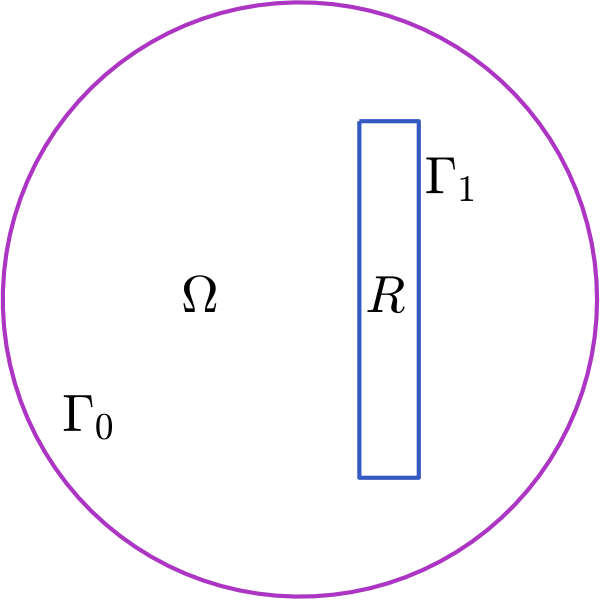
//  Data of the problem
//
real x0 = 0., y0 = 0., x1 = 10., y1 = 10.;     // corners of R
real x0B = 4., y0B = 4., rB = 1.;              // center and radius of the ball

func a11 = (1+x*x);                            // the components of A(x,y)
func a22 = (1+y*y);
func a12 = x*y;
func c   = 1.;                                 // the function c
func f   = 10.*(x*x-5.*y*y);                   // the function f
func u0  = 44.*(x*x+5.*y*y);                   // the function u_0
func alp = .1*(y*y-x*x);                       // the function \alpha
func h   = 3.4*(x*x-5.*y*y)*(y*y-x*x);         // the function h

//
//  Description of the boundary
//
//  Sides of the square
real mx = x1-x0, my = y1-y0,  pi2 = 2.*pi;
int nx = 30, ny = 30, nB = 30;              // mesh data
int L2 = 5, L1 = 9;                         // the labels: outer, inner
border C21(t=0.,1.){ x = x0+mx*t;  y = y0;      label=L2;}
border C22(t=0.,1.){ x = x1;       y = y0+my*t; label=L2;}
border C23(t=0.,1.){ x = x1-mx*t;  y = y1;      label=L2;}
border C24(t=0.,1.){ x = x0;       y = y1-my*t; label=L2;}
// boundary of the ball:
border C1(t=0.,pi2){ x=x0B+rB*cos(t); y=y0B+rB*sin(t); label=L1;}
plot(C21(nx)+C22(ny)+C23(nx)+C24(ny)+C1(-nB), cmm="The boundary", wait=true);

//
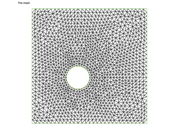
//  Mesh
//
mesh Th = buildmesh(C21(nx)+C22(ny)+C23(nx)+C24(ny)+C1(-nB));
plot(Th, cmm = "The mesh", wait=true);

//
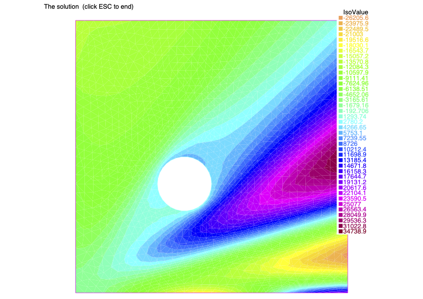
//  The Finite Element space and functions
//
fespace Vh(Th, P1);
Vh u, v;                                   // u: unknown,  v: test function
Vh ch = c, fh = f;                         // pde coeffs.
Vh a11h = a11, a22h = a22, a12h = a12;     // pde coeffs.
Vh u0h = u0, alph = alp, hh = h;           // boundary and initial cond. functions.s
//
//  The problem
//
problem CoefElliptic(u,v) = 
          int2d(Th)( a11h*dx(u)*dx(v) + a22h*dy(u)*dy(v)
        + a12h*(dx(u)*dy(v)+dy(u)*dx(v)) + ch*u*v)            // bilinear, PDE
    + int1d(Th,L2)(alph*u*v)                             // bilinear, Fourier
        - int2d(Th)(fh*v)                                     // linear, rhs
        - int1d(Th,L2)(hh*v)                                 // linear, Fourier
        + on(L1,u=u0h);                                      // Dirichlet data
    
CoefElliptic;
plot(u, nbiso=40, fill=true, value=true, 
      cmm = " The solution  (click ESC to end)", wait=true);

Anna Doubova - Rosa Echevarría - Dpto. EDAN - Universidad de Sevilla